The Chi-Square Distribution

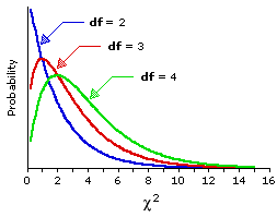
Throughout Chapter 8, the normal distribution was looked at when assessing situations, hypotheses and probabilities. However, the X² distribution, known as the chi-square distribution is just as effective as the normal distribution. The X² (chi square, pronounced kai-square) distribution is a continuous probability distribution that is widely used in statistical inference. In fact, it is closely related to the standard normal distribution; in that if a random variable Y has the standard normal distribution then Y² has an X² distribution with exactly one degree of freedom. Similarly, if Z₁, Z₂, …, Z_k are independent standard normal variables, then Z₁² +  Z₂² …+ Z_k² has an x² distribution with exactly k degrees of freedom. For the x² distribution, the mean is equal to the degrees of freedom, while the variance is twice the degrees of freedom.  As you see a visual representation, you will notice that as the degrees of freedom increase, the x² distribution will start looking like the normal distribution. Furthermore, the x² function with one degree of freedom is largely positively skewed, but as the degrees of freedom increases, the skew-ness of the graph begins decreasing.  The chi-square is a statistical test, which is commonly used to substantiate the null hypothesis, or to affirm the alternate hypothesis. It is often used when trying to determine the “goodness of fit” between the observed and recorded pieces of data and the expected outcomes (empirical vs. theoretical). Should there be a large difference between the expected and actual data; a large Chi-square value will result, indicating that there is a significant difference between the original hypothesis and the actual data. Before I lose you as a reader in this annihilation of words, (I hope I still have your undivided attention at this point), let me show you an example pertaining to the goodness of fit for a binomial distribution.

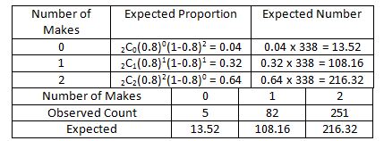
In several instances, we can use an x² test to verify or disprove the null hypothesis that the data comes from a specific parametric distribution (e.g. Binomial, Poisson, normal). As an example, suppose that a sports journalist claims that Michael Jordan’s free throw successes follow a binomial distribution with a success rate of 80%. Assume that the observed data over two seasons is as shown in the table below (take into consideration that the total number of free throw pairs is 338, and that each attempt consists of two free throws).

In words, on five occasions Michael Jordan missed both free throws during the two seasons, while scoring one out of two free throws on 82 occasions. He did also score both free throws on 251 occasions. In this instance, the H₀ is that Michael Jordan’s number of successes on two free throws follows a binomial distribution with a success rate of 80%; while the alternative hypothesis claims that the distribution differs from the null hypothesis in some manner. There are two situations in which the null hypothesis could be discredited; a) binomial distribution is reasonable, but the probability is wrong, or b) the binomial distribution is incorrect because free throws are not independent, but the probability of success is corrected. Now, let us calculate the expected proportion and the expected numbers if the null hypothesis was true.

Through the table shown above, we can see that there are several occasions where the expected value differs from the observed value. Based on the hypothesis, it was expected that Michael Jordan would only make 216.32 pairs of free throws; however, in reality he made 251. Similarly, the values between the expected number (based on the hypothesis) and the theoretical values differ. Through the naked eye, it is easy to point out that differences are witnessed in the two sets of data. However, is the difference statistically different? Can we reject the null hypothesis? Instead of using the normal distribution, we proceed to test the hypothesis using the chi-square method.

The formula for determining the chi-squared is as follows: the values that are observed are subtracted by the values that are expected, and then squared. The expected number then divides that expression. The formula is applied over all cells (in this case, 0, 1, 2 makes).

Through this, we can see that the chi-squared test statistic is equal to 17.26. Subsequently, the “p” value must be obtained. To begin with, the degrees of freedom are required and are obtained by subtracting one from the total number of cells (in this case, 3). That makes the division of freedom equal two. There are two ways in which we can calculate the “p” value; we can either draw the chi-square distribution with a degree of freedom of two, or then look for the values based on our chi-squared test statistic, or we can use an online calculator. Take into consideration that the larger the value of the test statistic, the greater the evidence against the null hypothesis. The “p” value is the probability of attaining values greater than the chi-squared test statistic (to the right of the value, on the graph). The larger the value, the harder to prove the hypothesis insignificant and inaccurate. In this instance, the “p” value generated by an online calculator is 0.00017866; it indicates a strong rejection towards the null hypothesis. Because we have obtained incriminating evidence that the hypothesis is not true, our work remains unfinished. As stated above, there are two possibilities in which the hypothesis can be incorrect, and it is necessary to test which of the possibilities is the underlying reason why the null hypothesis was rejected.

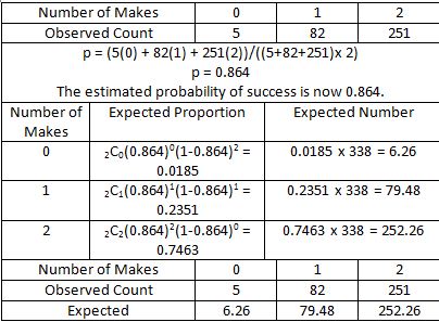
In practical situations, the ambiguous nature of the parameters is prevalent, and often, the available data is required to obtain these parameters. So for this case, let us assume that the parameters are not provided, and that we have to form them. For now, the null hypothesis can be reworded to state, “Michael Jordan’s number of successes on two free throws follows a binomial distribution” (notice that the statement does not contain any success values).  Let us then, estimate the probability that he made free throws.

After calculating the expected numbers based on the estimated probability that he made sets of free throws, we can immediately notice the close nature of the expected and observed count of Michael Jordan’s free throw shooting over two seasons.  Similar to the previous situation, we must calculate the chi-squared test statistic based on the new set of values. In this instance, the value of the test statistic is 0.34. Once again, the “p” value is required to determine whether the null hypothesis can be accepted or not. Therefore, there is a need to determine the degrees of freedom for the data set. While it may be quite enticing to say that the degree of freedom is two, there is a slight catch. Because we estimated the initial parameter for the data (finding p = 0.864), we have lost an extra degree of freedom. Therefore, the degree of freedom for this instance is one.  After using the online calculator to find “p”, or plotting the chi-square distribution with one degree of freedom, you will find that the value of p (area under the curve to the right of 0.34) is approximately 0.56. Since this is a large p-value, it indicates a strong approval for the null hypothesis. In conclusion, the null hypothesis was tested and approved as noticed through the large p-value because there is no evidence that Jordan’s true distribution of successful free throws differs from the binomial distribution.

In this way, the chi-squared method of either accepting or rejecting hypotheses is quite useful, given a set of data and a null hypothesis. The nature of the chi-squared method is similar to the other methods of verifying hypotheses, and offers an alternative manner to prove the same point.

Hope you as a reader, enjoyed reading all eight posts about Data Management in Mathematics. For now, this is the last post in the series, however, stay put for more in the future. Happy Reading 🙂

Before signing off, a special shout out to the following people; the creators of Daum Equation Editor (the program is a lifesaver), my entire Data Management class, Ms. Mark (my Data Management teacher), WordPress  and all you readers, followers, commentators and math enthusiasts out there.

Peace out xx

 

 

References:

http://www.colby.edu/biology/BI17x/freq.html
http://www.danielsoper.com/statcalc3/calc.aspx?id=11
http://statistics.unl.edu/faculty/bilder/categorical/Chapter1/Section1.2.pdf
http://www2.lv.psu.edu/jxm57/irp/chisquar.html
http://www.youtube.com/watch?v=O7wy6iBFdE8

The Multinomial and Poisson Distributions

As you and your friend travel one thousand miles to watch a series of Barclays Premier League football, the two of you deliberate the probability distributions for the possible results over the five game series. Conversely, it hits you right in the face, at MDM4U in school, you learnt calculating probability distributions for binomial circumstances, but football always encompasses a draw. You could manipulate the probabilities and count a “draw” as a loss, but would that really be a representative probability distribution? Undoubtedly not, unless you or your friend were rooting for one team so badly, that any result against them counted as a loss.

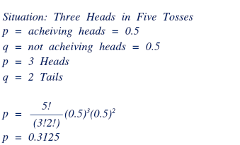
In class, Bernoulli trials in connotation with binomial distributions were conferred. As a reminder, let us take the time to revisit Bernoulli trials and binomial distributions. Bernoulli trials are recurrent, independent, indistinguishable trials measured in terms of success or failure. Several examples of independent trials include tossing a coin one hundred times, rolling a pair of dice, or pass and fail situations.  Binomial distributions are probability distributions where a definite outcome is anticipated, and where there are two possible results; success or failure. The probability of success is denoted as p, while the probability of failure is denoted as q. The sum of these two probabilities, must, in all situations be equal to one.  Let us take an example; what is the probability of tossing exactly three heads out of five tosses? The first step is to determine the success and failure, along with the probabilities and desired number of successes and failures, respectively. Therefore, the probability of achieving exactly three heads in five tosses is 0.3125 (10/32).

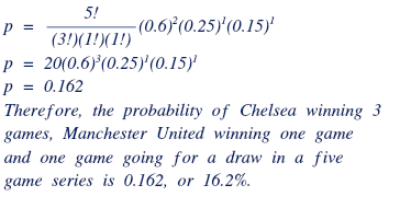
Going back to the football example, the situation of a draw is not covered by a binomial distribution, so, what do we do? Instead of using the binomial distribution, where there are two outcomes (success and failure), we proceed to using the formula for multinomial distribution, which allows infinite (n) outcomes, as long as the probabilities for (n-1) outcomes are defined, and the number of desired outcomes are also defined.  Suppose you were attending the game series between Chelsea and Manchester United, the probability of Chelsea winning is 60%, while the probability of Manchester United winning is 25%. The probability of a draw is the remaining 15%. If the series was five games long, what is the probability of three Chelsea wins, one Manchester United win and one draw? And what is the number of expected Chelsea wins, Manchester United wins and draws in the five game series?

The first step towards solving this issue is to gather the formula, and identify all the values associated with it. The formula for multinomial distributions is similar to that of the binomial distributions, with the only difference being an added outcome, denoted as “r” or “n₃”. In the football instance, n equals to five, because the game series is five matches long. The desired outcomes are three Chelsea wins (probability of Chelsea winning is 60%), one Manchester United win (probability of Manchester United winning is 25%),and one draw (probability of one match going for a draw is 15%). Subsequently, the values are to be entered into the formula and calculated based “on the order of operations”. After doing the above mentioned, the probability of Chelsea winning three games, Manchester United winning one game and one game stalemated, is attained, and is found to be 0.162 (or 16.2%).

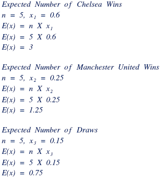
However, only parts of your queries are answered. As a football fanatic, you still do not know how many games your team is expected to win, or how many draws are expected to be part of the series? Recall that the formula for obtaining the expected number of successes in a binomial distribution was simply n x p (where n was the number of times the experiment/event occurred, and p was the probability of success). Similarly, the expected value for the number of desired outcomes can be obtained by multiplying the number of events/experiments by the probability of the desired outcome.

In the situation of the football series, the probabilities are 60%, 25% and 15% respectively, while the number of games occurring within the series is five. As a result, the expected values for the series are three Chelsea wins, one Manchester United win, and one draw.  In summary, situations where the number of outcomes are greater than two require more than a binomial distribution, hence the multinomial distribution is an effective manner in which the probabilities for situations that include more than two possible outcomes. Similarly, the expected value can also be calculated for these situations. The multinomial distribution can easily be used in situations like chess, stock prices, sporting events, and any other situation involving more than two possible outcomes.  However, what about situations in which rates are involved?

Over a century ago, French mathematician Simeon-Denis Poisson developed, what is known today as the Poisson distribution. There are several uses for the Poisson distribution. For instance, this style of distribution can be used to approximate the binomial distribution if the value of p is miniscule, but the value of n is extremely large. However, the more common use of the Poisson distribution is when an average rate of occurrence is given. It is especially used when the mean number of successes (predetermined outcome) is given, and the probabilities of various numbers of successes are required. By definition, the Poisson distribution is a discrete probability distribution for the counts of events that occur randomly in a given interval of time (or space). The Poisson distribution only works if the events are independent. The formula for the Poisson distribution is shown below:

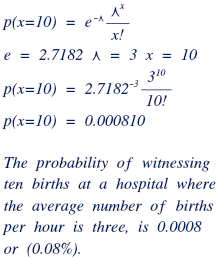
With regards to the Poisson distribution, the mean is equal to λ, while the standard deviation is equal to the square root of the mean.  As an example, you were tasked with  calculating the probability of observing 10 births in a given hour at the hospital, with the average rate of births per hour at the hospital being only 3. The first step is to provide a let statement, that x equals the number of births in a given hour.  Consequently, a Poisson distribution statement must be written. The general formula for that is X – Po(λ). Therefore, the general statement for this instance is X – Po(3). The mean of the births per hour at the hospital is 3, while x is 10.  After inputting all the information into the formula, you would realize that the probability of the desired outcome is 0.08%.

In summation, where the binomial distribution is unable to provide probabilities for situations, the multinomial distribution can be used when the number of outcomes exceeds two, and the Poisson distribution can be used when rates are provided, or the probability is too small and the sample  is too big to use the binomial distribution.

References:
http://www.youtube.com/watch?v=tx9wspMQvoY
http://www.statlect.com/mddmln1.htm
http://warnercnr.colostate.edu/~gwhite/fw663/MultinomialDistribution.PDF
http://www.math.uah.edu/stat/bernoulli/Multinomial.html
http://onlinestatbook.com/2/probability/multinomial.html
http://ncalculators.com/math-worksheets/poisson-distribution-example.htm
http://ncalculators.com/statistics/poisson-distribution-calculator.htm
http://easycalculation.com/statistics/learn-poisson-distribution.php
http://www.stats.ox.ac.uk/~marchini/teaching/L5/L5.notes.pdf
http://onlinestatbook.com/2/probability/poisson.html

A Multiple Linear Regression… “Wait what? Did I read that correctly?”

Regressions are mathematical processes in which relationships between variables are observed. There are several types of regressions that can be conducted on the data, namely; linear, polynomial, logistic, exponential, power, etc. By definition, a linear regression is the technique for finding the mathematical relationship between dependent and independent variables.  It finds the line of best fit for the data with a mathematical approach, and is only dependent on the data, without any human interaction and involvement. Linear regressions are essential because they allow future predictions to be made based on the data. However, the real world is complex, and often, it is hard to find a relationship between one dependent variable and one independent variable because there is a possibility of several factors being involved, or required for a solution. In class, we went over how a correlation does not always imply cause and effect. By using the concept of multiple regression, the common cause factors can be mathematically represented within the regression. The original least squares method of developing a linear regression is perhaps the most widely used type of regression for predicting the values of one dependent variable from the independent variable; however, it is also widely used to predict the value of one dependent variable from one or more independent variables. When that is the situation, the process is termed as a multiple linear regression. One of the more common examples of a multiple linear regression pertains to job satisfaction, wherein several variables such as salary, years of employment, age, gender and family status might influence one’s job satisfaction.

The steps in forming a multiple regression are almost the same as forming a linear regression. To begin with, you must form the research hypothesis followed by the null hypothesis. Next, you should assess each variable independently, and obtain the measures of central tendency and measures of spread. Also, question whether the variable is normally distributed or not? Then, assess the relationship that each independent variable has with the dependent variable, and determine the correlation coefficient. Are the two variables related? Next, assess the relationship that all of the independent variables have with each other, and create a correlation coefficient matrix for all of the independent variables. Furthermore, it is vital to determine whether the independent variables are too highly correlated with each other? An effective way to do this is to form a correlation matrix, one which describes the effect of each variable on the other, taking into consideration significance and the Pearson coefficient.  Consequently, the regression equation must be formed. This is often done using the aid of technology due to the strenuous and difficult process to come up with the equation. Following that, the correlation coefficient is analyzed and appropriate decisions are made based on the hypothesis. However, despite knowing all the steps involved in conducting a multiple regression, you must still be wondering what the equation actually looks like.

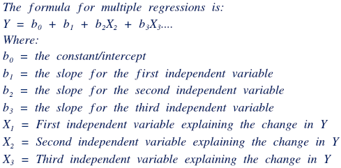
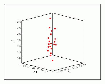
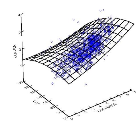
So for instance, you were trying to determine someone’s height, after completing puberty. In this case, said person’s height would be “Y”, because the value was dependent on other variables and factors. On the other hand, B₁ could represent the mother’s height, and the effect that has on a person’s height while X₁ would be a certain mother’s height, if we were to determine the height of their child. Likewise, B₂ and X₂ would represent the father’s height. The third independent variable could represent one’s gender, and be a binary variable. For instance, you would let females be represented by a zero, and males be represented by a one. Lastly, the constant, could perhaps be the average height of people before puberty. Consequently, you would compile all the pieces of data in a computerized program for the formation of a regression model, which would accurately depict the situation, because the process in which the regression is to be developed is extremely rigorous and time-consuming, which is why technology is preferred (often, the SPSS software is used).  A visual representation of a multiple regression graph composed of two independent variables and one dependent variable is shown. As you may notice, the scatter plot is produced three-dimensionally, because there are three variables involved in this correlation. If there were four variables involved, perhaps a tetrahedron shaped graph would be composed, in order to provide a visual representation of the data.

However, despite the fact that the multiple regression is effective in determining relationships, and explaining the changes in data that occur because of certain independent variables, there are several issues attached to the process of multiple regressions. For one, if the data cannot be modeled by a linear graph, then a multiple regression is literally pointless, as it will not be able to provide any inference. Moreover, the issue with performing a multiple regression is the added pieces of data that are required and need to be managed. With single linear regressions, a strong correlation would require at least fifty pieces of data, however, due to the added independent variables, it would be reasonable to attain at least twenty more pieces of data per variable added. In addition, variables that do not significantly contribute to the effect of the multiple regression should be eliminated as their effects on the regressions are minimal. Consequently, the issue of multicollinearity arises when variables are added to the correlation. This occurs when two or more of the independent variables are highly correlated to each other. If a 0.75 correlation coefficient is noticed or indicated, there is an enormous probability that an issue with multicollinearity will arise. If the two variables are highly correlated, they are basically measuring the same phenomenon, and when one enters the regression equation, it is able to explain the variance in the dependent variable. This leaves little for the second independent variable to do, and often, could cause a potential skew in the regression due to multicollinearity. On the other hand, despite there being the potential for problems with multiple regressions, in this world where there are several common cause factors which could affect correlations, the option to include secondary independent variables provides researchers and analysts with strong advantages, in order to reaffirm their hypotheses.

 

References:
http://www-stat.wharton.upenn.edu/~stine/stat621/handouts/MultRegr.practice.pdf
http://www.palgrave.com/pdfs/0333734718.pdf
http://people.stern.nyu.edu/wgreene/Statistics/MultipleRegressionBasicsCollection.pdf
http://www.csulb.edu/~msaintg/ppa696/696regmx.htm
http://www.stat.yale.edu/Courses/1997-98/101/linmult.htm

Absolute Mean Deviation

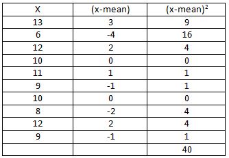
For a long time, I have not only debated with myself, but with others about standard deviation. To me, the formula makes as little sense as pre-calculus would do to an elementary student. Why would you want to square all the differences between the x values and the mean, and then find an average of those, and then square root the average? When you could just as simply find the difference between x values and the mean, convert them all to positives and then find the average between them? Before I proceed degrading the standard deviation any more, and promoting the absolute mean deviation, let me, take the time to explain the two. The standard deviation is a measure of spread, one of the most common ways in which a dataset can be analyzed. The process of attaining the standard deviation is by summing the squared values of each measurement’s deviation, dividing that value by the total number of measurements and then taking the positive square root of the result. Assume that you have a dataset of ten positive integers with a mean of ten:  13,6,12,10,11,9,10,8,12,9

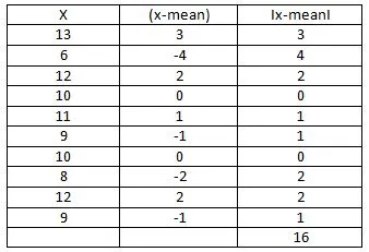
In this instance, the sum of the squared deviations equals 40. The next step is to divide forty by the number of measurements, in this case 10. That leaves us with four, the variance value. The standard deviation is the positive value of the variance square-rooted, which then indicates that the standard deviation for this data set is two. On the other hand, the process of obtaining the absolute mean deviation is much simpler. The first step is to identify the mean, and subtract all of the x values from the mean (the same step was conducted to find the standard deviation). However, instead of squaring the numbers, the absolute mean deviation requires all deviations to be positive using absolute values. After which, an average of the positive deviations are taken yielding in the absolute mean deviation. Once again, assume that you have a dataset of ten positive integers with a mean of ten:  13,6,12,10,11,9,10,8,12,9

The sum of the deviations equals 16. Following that, the sums of the deviations are to be divided by the number of measurements, in this case 10. Hence, the absolute mean deviation is 1.6 for the above-mentioned dataset. Seeing, as it required lot less time and effort to produce the absolute mean deviation, as opposed to the standard deviation; why is the standard deviation still preferred to the absolute mean deviation? The formula, and an example of the absolute mean deviation is herewith shown below:

The mean deviation is much easier for newer researchers to understand intuitively than the standard deviation, because it is simply the average of the deviations. It has a clear meaning; the absolute mean deviation is the amount by which particular values differ from the mean on average. The standard deviation, however, does not have a clear meaning.  In 1914, a British astrophysicist known as Arthur Eddington pointed out that calculating the absolute mean deviation is not only easier, but also more accurate than the standard deviation, especially since the margin for error in his field was greater. He claimed that it worked especially better with empirical data than the standard deviation did.  However, Fisher, who believed that the standard deviation was more efficient than the absolute mean deviation under ideal circumstances, formed a counterargument. What Fisher failed to realize, is that it is nearly impossible for a measurement to be entirely error free, and hence the absolute mean deviation would work better in most situations. Moreover, scientists like Fisher have often tried to compare the standard deviation (population) versus standard deviation (sample) with absolute mean deviation (sample) versus the standard deviation (population). Comparisons like that often lead to inaccurate findings. Other social scientists and scientists believe that the absolute value symbols used in the absolute mean deviation formula ensure that it is much harder for the formula to be algebraically manipulated, as opposed to the standard deviation formula.

On the other hand, there are several situations where the absolute mean deviation is preferred, and there are several advantages attached to using the absolute mean deviation. In situations where some of the measurements do contain slight errors, the distribution is not perfectly normal, and when further analysis needs to be conducted, the absolute mean deviation is easier to obtain and easier to understand. This translates into the fact that for the standard deviation to be more effective than the absolute mean deviation, the data would have to be error free, and without any contamination. To begin with, utilizing the absolute mean deviation reduces the potential of errors within the dispersion, because it gives us less of a distorted view of the spread. The standard deviation requires the subtraction of the mean from each x value to be squared, ensuring that each unit of distance from the mean is exponentially (rather than additively) greater. Make no mistake; the act of square rooting the sum of the squares does not effectively and completely eradicate this bias. This serves as the primary reason why (in example 1) the standard deviation is 0.4 units greater than the absolute mean deviation.

The works of Barnett and Lewis discovered that the advantage in efficiency and effectiveness that the standard deviation is dramatically reversed when even an error element as small as 0.2% (2 error points in 1000 observations) is found within the data. In most realistic situations, there is bound to be at least a miniscule percentage of error elements, and as seen in the works of Barnett and Lewis, the advantage of the standard deviation over the absolute mean deviation is immediately reversed when that is the case. In addition, an assumption, which underlies the superiority of the standard deviation, is that it involves working with samples selected from a fixed population. However, that will not always be the case, especially in situations when working with the population, with a non-probability sample, or with a probability sample with considerable amounts of lack of responses. In each of these situations, it is acceptable to calculate the variance of certain values in comparison to the mean; however, forming the population standard deviation is improper and inaccurate. Lastly, the practice of removing outliers has been immensely lopsided with the use of the standard deviation. Because of the large bias and inconsistencies faced with squaring and then square-rooting data in order to produce the SD, the exclusion and deletion of outliers has often occurred, despite there not being a need for it to occur.  Regardless of the importance of the data, those in education are often told to remove or ignore valid measurements with large deviations because they negatively influence correlations. However, the fault in that, is that the large nature of the deviations are only exaggerated by the production of the SD, and that perhaps the MD would not result in such large deviations and hence the removal of key pieces of data. Moreover, extreme values (not exaggerated extreme values) are quite essential in a variety of natural and social phenomena, including but not limited to city population growth, income distributions, earthquakes and traffic jams. As a result, in practice and in empirical situations, the absolute mean deviation (MD) should be preferred to the standard deviation (SD) due to the easiness in which the former can be utilized, and the fact that it has been proven more effective and accurate.

Especially since most of the calculations conducted today are formed using formulas and are outsourced to technology, the difficulty in using absolute values is dramatically reduced, and simplified. Given that, the SD and MD nearly perform the same tasks, and in most situations, the MD tends to be more accurate, it would only make practical sense for researchers, scientists and social scientists to take the simpler route in the absolute mean deviation. Complexity could be the cause of failure when performing correlations.

References:

http://www.math.unb.ca/~knight/BasicStat/absdev.htm
http://www.mathsisfun.com/data/standard-deviation.html
http://investwhy.com/showthread.php?171397-standard-deviation-vs-mean-absolute-deviation
http://www.leeds.ac.uk/educol/documents/00003759.htm

The Cayley Hamilton Theorem & Its Applications

As you walk in for the final math exam that determines whether you graduate high school or not, what is your greatest fear? Me being me, my greatest fear is to do with my graphing calculator and me forgetting to bring it, yes, me and my ever-so precious graphing calculator. There would be a really high chance of me failing that particular exam without my savior, and that would mean me not being able to graduate. Thankfully, that situation has not occurred to me (touches wood), and I hope that it won’t happen to you either.  However, let’s assume the worst case scenario.  Seeing as we are in a Data Management Class, it is nearly guaranteed that matrices are going to be part of the exam. Most likely, you will have to a) find the inverse of it or b) raise it to a fairly large power with the aid of your graphing calculator. Oh wait, that’s right, you don’t have one. Well, what do you do? Enter the Cayley-Hamilton Theorem.

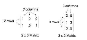
Arthur Cayley and William Rowan Hamilton, two mathematicians discovered a unique feature pertaining to matrices. In case you have no clue about what matrices are, let me enlighten you. In the complex, dynamic and ever-changing world of mathematics, a matrix (plural form matrices) is a rectangular array of numbers, symbols or even expressions arranged into rows and columns. Each individual number/symbol/or expression is known as an element or an entry. A matrix with two rows and three columns is referred to as a 2 x 3 (row by column) (read as two by three) matrix. Matrices are very useful because they provide a manner in which you can organize and manage large amounts of data. Furthermore, once certain data is inputted into a matrix, it can be manipulated in a variety of manners in order to acquire different types of data or to conduct a more developed analysis on the data. The image shown directly below provides two examples of matrices, a 2 x 3 matrix and a 3 by 2 matrix.

An important thing to remember is that the Cayley-Hamilton Theorem can only be used with square matrices. What does this mean? The matrix must have the same number of columns, as it does rows. E.g. a 2 x 2 matrix is classified as a square matrix, and so is a 3 by 3 matrix. The Cayley-Hamilton Theorem (henceforth referred to as CHT) states that every square matrix satisfies its own characteristic equation. In simpler words, if A is given n x n matrix and I_n is the identity matrix in the form of n x n, the characteristic polynomial of A is defined as: (see image below). In this equation, the “det” refers to the determinant operation.  Moreover, as the entries of matrix A are (linear or constant) polynomials in λ, the determinant is also an n-th order polynomial in λ. The Cayley-Hamilton Theorem also states that substitution for the matrix A in this very polynomial function will result in the zero matrix.

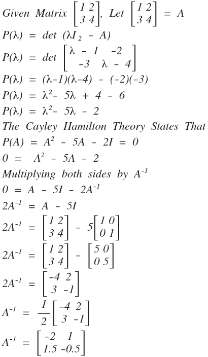
To begin with, let us attempt to derive the inverse of a two by two square matrix using the Cayley Hamilton Theorem. The first step is to define the matrix as A. Next, you must compute the characteristic polynomial, the method in which to do this differs based on the size of the matrix. Due to time constraints, this blog will only cover how to calculate the characteristic polynomial for two by two matrices. For information on how to calculate the characteristic polynomial for a three by three matrices, see: http://www.youtube.com/watch?v=FZz-Q-KBlpE. In this case, the characteristic polynomial is calculated by finding the determinant of the two by two matrix. Term A₁₁ and A₂₂ are subtracted by λ, and then multiplied together. That expression is then subtracted by the multiplication of the negative values of term A₁₂ and term A₂₁. After coming up with the characteristic polynomial, you then need to apply the CHT, and multiply both sides by A^-1. From then onwards, it is a matter of isolating the inverse of matrix A.

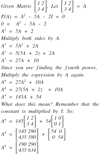
Since we have already developed the characteristic equation for a two by two matrix, let us use the same equation and the same matrix. In this case, imagine that you have been asked to raise matrix A to the power of four. Well, you don’t have your calculator. So, what do you do? Once again, you can use the Cayley Hamilton Theorem. In this case, we are looking for matrix A raised to the power of four, meaning the end expression should be in terms of A⁴. Thus, we first multiply both sides by A, so that the expression is in terms of A³. Then, you must replace A² with its expression, as defined in the working. The same steps are then repeated until the left side of the equation reads A⁴ and henceforth the highest degree of terms is one. Once that is done, simply recall that the constant is multiplied by the identity matrix and simplify the expression.

Once you have understood the process for two by two matrices, doing it for three by three matrices is like applying butter to bread. The process is for the most part, extremely similar. The only challenge that a three by three matrix presents pertains to developing the characteristic polynomial given a matrix. The challenge for you, as a reader is to develop that formula, as well as one for the nth by nth matrix.

Sources:
http://www.youtube.com/watch?v=uMBsABTWLI8
http://www.youtube.com/watch?v=FZz-Q-KBlpE
http://www.youtube.com/watch?v=RgQFaK28sB
http://www.youtube.com/watch?v=mn6198-LLfw
http://www.youtube.com/watch?v=1-nS-h5MRZM

Poker: 100% Skill & Numbers and 50% Luck

Walking into a casino, you may have told yourself the following: “winning and losing at a casino is solely dependent on luck”. On the contrary, success in most card games at the casino is split between luck and your competencies at understanding numbers. For all it may be, poker, whether five or seven card, whether one or multi deck is a number’s game.  Anthony Holden, the author of Big Deal once said “The good news is that in every deck of fifty-two cards there are 2,598,960 possible hands.  The bad news is that you are only going to be dealt one of them.”

With poker, a common misconception is that the more decks that are involved, the harder the chances of winning. That, for the most part, isn’t true. When gambling, the higher the odds you receive, the lower the probability of the desired events occurring.  Gambling odds are not odds in favor, but instead are odds against, which is the probability of the event not occurring divided by the probability of the event occurring. This entry aims to a) derive the odds pertaining to each hand in five card poker with one, two, three, and four decks being involved and b) articulate the different probabilities that arise when dealing with single and multiple decks, namely, two, three and four decks.

To begin with, let me take the time to explain five card poker (often referred to as “five card draw”), which includes a dealer. Each player, including the dealer is dealt out five cards. Your goal is to have a hand better than the dealer’s. There is only one round of gambling (in most cases), which occurs before the hand is dealt. You can put as much money on the table, and should you win, the payout will be your money multiplied by the odds predetermined by the casino. After receiving your hand, you have the choice of exchanging a maximum of three cards for a maximum of three cards, dealt directly from the deck. Should you have a hand better than the dealer, e.g. four of a kind vs. two pair, you win your bet against the dealer, and will be paid the odds of a four of a kind multiplied by the amount of your bet.  Before I lose you as a reader and this entry progresses, it is vital that you understand the types of hands involved in poker.

Consider this scenario, you are playing poker in an underground den with one deck, amongst your five card hand; you have five spades, albeit in no definite order, your cards are A, 3, 6, 9, Q. You do not have a straight, but, your hand ensures that the probability of obtaining a royal flush inches closer to zero for everyone, including the dealer. The dealer says that you are allowed to bet during the game. The odds of you winning are substantially higher now, because there are only four types of hands that are superior to yours, but the probability of obtaining those hands are very remote and you can bet during the game. As a result, you may choose to raise the dealer, because your chances of winning are higher. By understanding the numbers well enough, you can make an informed decision whether you wish to raise, call, or, fold versus the dealer.  The table below shows you the approximate probabilities and odds for each type of hand in five card poker with one deck.

Mathematical Reasoning:

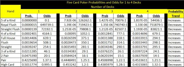
After seeing how the probabilities, and odds for each possible hand in five card poker with one deck was derived, the comparison of probabilities between one deck and multi deck five card poker will be shown in the following table.

As you can see from above, the probabilities of achieving most hands increases as you add more decks. Apart from straights and high cards, the probabilities of each of the hands increase, while the odds decrease. Yes, the payout odds for each of those hands also decrease, but there is a greater chance of you winning. So, what type of gambler are you, a greedy one bent on making the most amount of money, or a smart one content with just winning?

So, walking into a casino, will you still tell yourself the following: “winning and losing at a casino is solely dependent on luck”.  I certainly hope not because in most card games at the casino or even in your hidden gambling ring, success between luck and your competencies at understanding numbers. If you know the numbers and are allowed to make bets during the game, you may have a significant advantage over your opponent. The next challenge for you, as a reader or as a gambler would be to identify whether playing poker which involves larger hands (e.g. six card, seven card, etc.) increases your probability of winning. Poker, be it five or seven cards, is in large part a number’s game.

Phil Hellmuth once said, “I guess if there weren’t luck involved, I’d win every time”. He mastered the game of poker, ensured that he lost little, but still could never win a hundred percent of the time. It is often said “when a man with money meets a man with experience and skill, the man with the skill and experience leaves with the money and the man who had the money leaves with experience and skill”.

References:
http://wizardofodds.com/games/poker/
http://blog.contextures.com/archives/2009/01/16/calculate-a-ratio-in-excel/
http://www.math.hawaii.edu/~ramsey/Probability/PokerHands.html

The Trinomial Theorem and Pascal’s Tetrahedron

Like most situations, there are two ways in which you can look at things. Consider this situation with the idea of a coin. On one side, you can use the trinomial expansion theorem to determine the coefficients of terms within Pascal’s Tetrahedron. On the other hand, you can use the already existent Pascal’s Triangle to derive the coefficients in Pascal’s Tetrahedron and from then conduct the trinomial expansion with great ease. Think of it this way: you can use algebra to help you with geometry, but you can also use geometry to help you with algebra. Anyway, however, you look at it, you come to the same conclusion; Blaise Pascal’s level of ingenuity continues to rise with each passing day, as the patterns found in Pascal’s tetrahedron are just as fascinating as those found in the triangle.

The definition of Pascal’s tetrahedron (or triangular pyramid) is as follows: Pascal’s pyramid is a three-dimensional arrangement of the trinomial numbers, which are the coefficients of the trinomial expansion and the trinomial distribution”. The tetrahedron is a correspondent of the two-dimensional Pascal’s Triangle. The problem, with the tetrahedron is that it can be extremely hard to visualize because of its three dimensional nature. Another issue arises when you attempt to derive the trinomial coefficients that would fit in the tetrahedron. This is because of the inability to visualize the tetrahedron. To begin with, let us derive the first four layers (zero to three) of Pascal’s Tetrahedron, using algebra and expansion. This is done by firstly expanding each of the trinomials linearly, and then organizing them in a theoretically understandable manner, creating layers of Pascal’s Tetrahedron.

From the illustration shown above, you may notice the following: the last rows of each layer are synonymous with their respective rows in Pascal’s Triangle. For instance, as the illustration shows below, the last row of the fourth layer of Pascal’s Tetrahedron reads as: 1 3 3 1, which is the same as the fourth row in Pascal’s triangle.  In addition, you will also realize that the diagonals adjoining the vertices also read 1 3 3 1, which corresponds to the fourth row in Pascal’s triangle. Moreover, you will notice that each outline of the nth layer in Pascal’s Triangle is a binomial expansion of degree n. As we can see from the example shown below of the fourth layer of Pascal’s Tetrahedron, the left outline is a binomial expansion of (a+b)³, while the right outline is a binomial expansion of (a+c)³ and the bottom outline is a binomial expansion of (b+c)³. Each of them is highlighted in yellow for identification purposes. Furthermore, you may notice that the terms with the highest powers are situated at the vertices, because the coefficients of those terms are “1”. This is analogous to the binomial theorem which utilizes Pascal’s Triangle.

Another interesting pattern present in Pascal’s Tetrahedron that can be related to Pascal’s Triangle, is the sum of the terms within each layer. In Pascal’s Triangle, which was two-dimensional, the expression used to determine the sum of the row was (1+1)ⁿ, each “1” pertaining to the number of dimensions, this was then simplified down to 2ⁿ. Similarly, as we have added another dimension, the sum of the terms present in the nth layer of Pascal’s Tetrahedron is attained using the expression (1+1+1)ⁿ, which is simplified down to 3ⁿ.  Moreover, the number of terms in the nth layer is equal to (n+1)(n+2)/2.

Verification (1): The third layer of Pascal’s Tetrahedron has the terms: (1 3 3 3 6 3 1 3 3 1), which adds up to a total of 27. In this case, n = 3, because it is the third layer. Therefore, the expression which represents the sum of the terms of the third layer is 3³, which results in 27. This proves that the expression 3ⁿ can be used to determine the sum of the terms present in the nth layer of Pascal’s Tetrahedron.

Verification (2): Q) How many terms are present in the 5th layer of Pascal’s Tetrahedron.  A) n = 5, ((5+1) x (5+2))/2 = (6)(7)/2 = 42/2 = 21. By counting the number of terms in the 5^th layer of Pascal’s Tetrahedron, you will realize that there are exactly 21 terms, and that this formula works.

In order to visualize Pascal’s Tetrahedron, as well as try and come up with the coefficients for the trinomial theorem,  try and picture each the layers sitting on top of each other. Don’t feel like you are the only one struggling to picture this, I had issues too. You may wonder, don’t we just add the two numbers above, and come up with the corresponding coefficient. Well, unlike Pascal’s Triangle, this is slightly more complicated. In order to attain the next entry in the nth layer of Pascal’s Tetrahedron, you must sum the entries in the nth-1 layer that are touching it. Basically, the goal is to form an equilateral triangle, and sum the three numbers to get the next entry. In simpler terms, the sum of three adjacent numbers in the previous layers gives it a number in the consequent layer. However, if the third adjacent number falls outside the triangular layer, that number is represented as a zero (see blue and orange highlights). In the illustration shown below, the outcome, which is the term in the sixth layer, is highlighted in one color and the terms required to reaching that term are highlighted in the same color in the fifth layer.

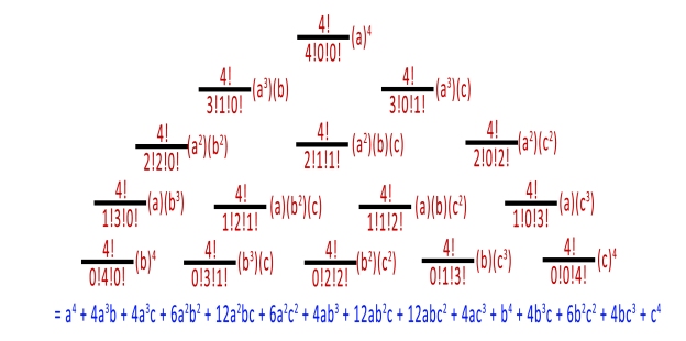
In class, we went over how to use Pascal’s Triangle’s coefficients and relate them to the binomial theorem. The formula, that is used determine the trinomial coefficients and exponent values in Pascal’s Tetrahedron, is quite similar to the one used to determine binomial coefficients and exponent values in Pascal’s Triangle. For binomial expansions where (a^m + b^k) ⁿ, m + k must equal n, at all times, while the value of the coefficient was either taken directly from Pascal’s Triangle or calculated using the formula shown below, where n was the value of the degree (which corresponded to the row number) and m was the term number. For trinomial expansions, in the form of (a^m+ b^k + c^l)ⁿ, for all terms, m+k+l = n, while the value of the coefficient can be derived using Pascal’s Tetrahedron or using the formula shown below, which is an extension of the formula used to determine binomial coefficients. In more mathematical terms, the value of the coefficient of Pascal’s Tetrahedron located at (n-m, m-k, k) which is the coefficient of the term a^n-mb^m-kc^k can be obtained using the trinomial coefficient formula shown below. The formula for the trinomial theorem is also shown below, and is partially, if not entirely composed of the formula to determine trinomial coefficients.

Putting Pascal’s Tetrahedron and The Trinomial Theorem To Work:

Question: Expand (a+b+c)⁴
Answer: There are two ways to do this. A) Derive the coefficients using Pascal’s Tetrahedron or B) Use the Trinomial Coefficients Formula to derive the coefficients.
Using Method B – Steps (See Solution Below):
1. Ensure that the highest powers of a, b, c each lie on the vertices of the triangle
2. Ensure that along the edges of either side, you are decreasing the value of (n-m) and increasing the value of either (m-k) or k.
3. For the base, ensure that the values of (m-k) decreases, while the value of k increases as you shift from left to right.
4. Fill in the exponents of a, b and c, in a similar fashion.
5. Compute and sum each of the terms to obtain the expanded form of (a+b+c)⁴.

Fun For You
a) Expand (a+b+c)⁷ using Method B (stated above)
b) Derive a formula for i) the number of terms for a multinomial element ii) the sum of the terms for a multinomial element iii) the coefficient formula for a multinomial expansion.

References:
http://www.math.rutgers.edu/~erowland/pascalssimplices.html
http://www.youtube.com/watch?v=OMr9ZF1jgNc
http://www.youtube.com/watch?v=k4z2Y8Y_r-M

Pascal’s Triangle: Cubic, Quartic and Sextic Numbers

According to Merriam-Webster, Pascal’s Triangle by definition is “a triangular arrangement of the binomial coefficients of the expansion (x + y)ⁿ for positive integral values of n”. In my opinion, the abovementioned is extremely depleted and vague definition of one of the greatest discoveries in the world of arithmetic. Pascal’s triangle is in itself a genius, a one-of-a-kind. It is a maze filled overloaded with patterns, and with each passing day that you study Pascal’s Triangle, you will find that the patterns within the triangle continue to increase. Call him conceited or vainglorious if you must, yet within yourself you very well realize that Pascal’s Triangle was aptly and well deservedly named after its compiler; Blaise Pascal.

In class, several patterns within Pascal’s Triangle were taught and/or discovered. These especially included patterns relating to the diagonals which portrayed triangular numbers as well as tetrahedral numbers. Based on that, many of us then connected the concept and discovered that the fifth diagonal was composed of pentatope numbers.  In addition, the concept of generating square numbers through the adding of two consecutive numbers belonging to the 3^rd diagonal (later known as the diagonal of the triangular numbers) in Pascal’s triangle was also touched upon.      Noticing, that it was possible to find square numbers within Pascal’s triangle, I wondered whether it was possible to find the cubic and quartic numbers using Pascal’s triangle.

It certainly was. You may have thought that since adding two consecutive triangular numbers yields in square numbers, shouldn’t adding three consecutive triangular numbers yield in cubic numbers. The answer is no. You may have then gone on and said, how about adding three consecutive tetrahedral numbers. However, even adding three consecutive tetrahedral numbers (see image to see the location of tetrahedral numbers) does not result in cubic numbers. With your second hypothesis, you are not entirely wrong; in fact it is almost correct.

Tetrahedral Numbers within Pascal’s Triangle

Square Numbers

In order to understand the formula required to yield cubic numbers with the help of Pascal’s triangle, it is vital that you understand how the formula for developing square numbers was established (see working below).  As we learned in class, square numbers are formed by combining two consecutive triangular numbers. But did we learn why? The formula for triangular numbers is as follows: n(n+1)/2. You will notice (after expanding the expression) that it one of the terms of the expression reads n²/2. This means that in order to reach n-squared, you need to add one consecutive triangular number; the (n-1)^th triangular number. When done so (as shown below), the end result is n-squared; the desired outcome. Therefore, the n^th squared number is equal to the n^th triangular number added to the (n-1)^th triangular number.

Working showing how Triangular Numbers that are found through the use of Pascal’s Triangle can be used in order to develop a formula for Square Numbers with the use of Pascal’s Triangle.

Cubic Numbers:

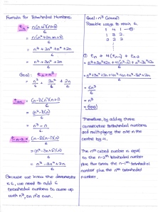
In the course, it was established that the formula for finding the nth tetrahedral number was n(n+1)(n+2)/6.  When expanded the formula becomes (n³ + 3n² + 2n)/6. Carefully look at the first term of that equation, it reads n³/6, this means that in order to get n³ completely isolated, you would need to add six tetrahedral numbers. Multiplying the equation by 6, doesn’t completely isolate n raised to the power of 3. As observed with the square numbers, two consecutive triangular numbers were added together. In this case, we would require the addition of three consecutive tetrahedral numbers. As a result, the formulas for the (n-1) ^th and (n-2) ^th tetrahedral numbers were derived. From the work shown below, you may notice that there were several ways in which you could combine the three consecutive terms so that you could reach a total of six tetrahedral numbers. However, the way in which you would do it in order to end up with an isolated n to the power of 3 would be to add three consecutive tetrahedral numbers, but multiply the one in the center by four. When done so (as shown below), the end result is n-cubed; the desired outcome. Therefore, the n^th cubic number is equal to the n^th tetrahedral number added to four times the (n-1)^th tetrahedral number added to the (n-2)^th tetrahedral number.

Working showing how Tetrahedral Numbers are used in order to develop a formula for Cubic Numbers via the use of Pascal’s Triangle

Hypothesized:  The n^th cubic number is equal to the n^th tetrahedral number added to four times the (n-1)^th tetrahedral number added to the (n-2)^th tetrahedral number.

Test:

• Let the n^th tetrahedral number be 35 (fifth tetrahedral number)
• Let the (n-1)^th tetrahedral number be 20 (fourth tetrahedral number)
• Let the (n-2)^th tetrahedral number be 10 (third tetrahedral number)

Working:

• (35) + 4(20) + (10)
• 35 + 80 + 10
• 125
• Cube Root (125)
• 5  (fifth cubic number)

Conclusion: The n^th cubic number is equal to the n^th tetrahedral number added to four times the (n-1)^th tetrahedral number and the (n-2)^th tetrahedral number as proved in the test conducted above.

Quartic Numbers:

According to the power of the product exponent law, an exponent raised to an exponent results in both of those exponents being multiplied. Consider the case: . Therefore, in accordance with the exponent laws, the n^th quartic number is equal to the n^th squared number to the power of two.

Sextic Numbers:

Similar to the case with the quartic numbers, according to the power of the product exponent law, an exponent raised to an exponent results in both of those exponents being multiplied. Consider the case: . Therefore, in agreement with the exponent laws, the n^th sextic number is equal to the (n^th cubic number) to the power of two.

A Cool Find:

You didn’t think that Pascal’s Triangle had run dry, now did you? In each row of Pascal’s Triangle, the first number is designated as the 0^th term of the row. Based on that, if the 1^st term of the n^th row is a prime number, all of the other numbers present within that row (aside from the ones) are divisible by n.

Fun For You:

a)      Develop a formula to find the n^th quintic number using Pascal’s Triangle.

b)      How can you use this formula to determine the n^th decic number?

c)       State two formulas that you can use to determine the n^th octic number? (Hint: Both require the use of exponent laws)